Attenzione!
La quasi totalità dei problemi numerici possono essere affrontati con algoritmi diversi, alcuni dei quali richiedono condizioni particolari. L'applicabilità del metodo scelto e la correttezza del risultato ottenuto devono essere verificati dall'utente.Attenzione!
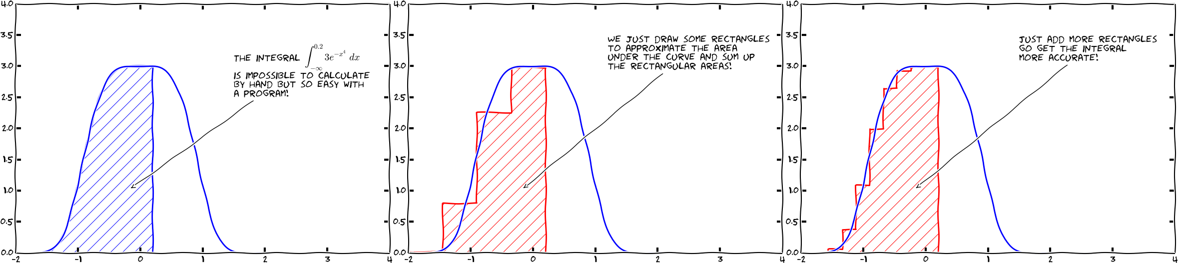
Qualunque manipolazione di una funzione nota deve partire dal grafico che guiderà i passi successivi. Nessun metodo per quanto potente è in grado di prendere sempre le decisioni corrette per una qualsiasi funzione il cui campo di esistenza e range di valori sono in linea di principio l'intero asse reale.- Quando si deve calcolare un integrale è opportuno fare il grafico della funzione integranda per controllarne il comportamento. Singolarità (per esempio valori di $x$ in cui $f(x)$ tende a più o meno infinito) oppure altri comportamenti irregolari, come quello di $f(x)=\sin(\frac{1}{x}$) nell'intorno di $x = 0$, sono estremamente difficili e talvolta semplicemente impossibili da trattare numericamente.
- La ricerca di zeri oppure di massimi e minimi richiedono un punto oppure un intervallo iniziale. Il modo più semplice per determinare questi valori è esaminare graficamente la funzione.
10.2 Integrazione numerica
(Svein Linge, Hans Petter Langtangen - Programming for Computations)
Scientific Python fornisce diverse routines di integrazione. Uno strumento di uso generale per calcolare integrali I del tipo
$$I=\int_a^b f(x) \mathrm{d} x$$è la funzione quad() del modulo scipy.integrate.
Prende in input la funzione f(x) da integrare (l'“integrando”) e gli estremi inferiore e superiore a and b. Restituisce due valori, (in una tuple): il primo è il risultato dell'integrale mentre il secondo è una stima dell'errore numerico del risultato.
from scipy import integrate
help(integrate.quad)
Ecco un esempio: $$I=\int_{-2}^{2} e^{\cos(-2 \pi x)} \,\mathrm{d} x$$
from math import cos, exp, pi
from scipy.integrate import quad

# funzione da integrare
def f(x):
    return exp(cos(-2 * x * pi))

# chiamata a quad
res, err = quad(f, -2, 2)

print(f"The numerical result is {res:f} (+-{err:g})")
Usando Numpy:
import numpy as np
def f_N(x):
    return np.exp(np.cos(-2 * x * np.pi))

res, err = quad(f_N, -2, 2)
print(f"The numerical result is {res:f} (+-{err:g})")
Si noti che quad() può prendere come parametri opzionali epsabs e epsrel per aumentare o diminuire l'accuratezza del calcolo (Usate help(quad) per maggiori informazioni). I valori di default sono epsabs=1.5e-8 and epsrel=1.5e-8. Per il prossimo esercizio, i valori di default sono sufficienti.
Integrazione su un intervallo infinito
def my_f(x):
    return 1/x/x

res, err = quad(my_f, 1, np.inf)
print(f"The numerical result is {res:f} (+-{err:g})")
Integrazione di una funzione che dipende da parametri
Talvolta la funzione da integrare dipende da dei parametri. Per esempio la velocità di un corpo che si muove in un campo gravitazionale costante è dato da $v(t) = g t + v_0 $
dove $v_0$ è la velocità a $t = 0$. Lo spostamento $y(t)$ può essere calcolato integrando questa relazione fra 0 e $t$
In questo caso la variabile su cui integrare deve essere al primo posto fra le variabili della funzione e i parametri addizionali vengono passati in una ntupla args:
from scipy.integrate import quad

def vel(t,v0):
    g = -9.81
    return g*t + v0

v0 = 10  # m/s
tf = 3  # s

y,err = quad(vel,0,tf,args=(v0,))
print(f"La posizione di un corpo che parte dall'origine con v0={v0} dopo {tf} secondi è {y} m")
Integrazione di una singolarità "integrabile":
def inv_square_root(x):
    return 1./np.sqrt(x)

res,err = quad(inv_square_root,0,1)
res,err
Integrazione di una singolarità "non integrabile":
def inv(x):
    return 1./x

res,err = quad(inv,0,1)
res
Integrazione con metodo dei trapezi
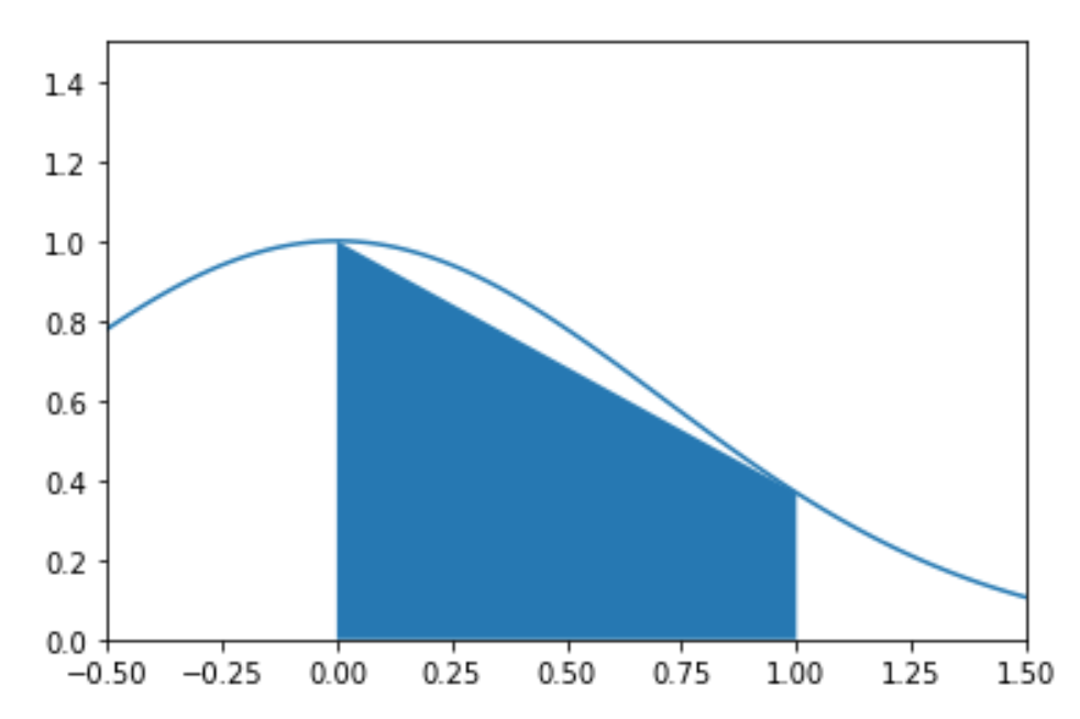
Un esempio di routine che integra una funzione usando il metodo dei trapezi:
# https://www.math.ubc.ca/~pwalls/math-python/integration/trapezoid-rule/

import numpy as np

def my_trapz(f,a,b,N=50):
    '''Approximate the integral of f(x) from a to b by the trapezoid rule.

    The trapezoid rule approximates the integral \int_a^b f(x) dx by the sum:
    (dx/2) \sum_{k=1}^N (f(x_k) + f(x_{k-1}))
    where x_k = a + k*dx and dx = (b - a)/N.

    Parameters
    ----------
    f : function
        Vectorized function of a single variable
    a , b : numbers
        Interval of integration [a,b]
    N : integer
        Number of subintervals of [a,b]

    Returns
    -------
    float
        Approximation of the integral of f(x) from a to b using the
        trapezoid rule with N subintervals of equal length.

    Examples
    --------
    >>> my_trapz(np.sin,0,np.pi/2,1000)
    0.9999997943832332
    '''
    x = np.linspace(a,b,N+1) # N+1 points make N subintervals
    y = f(x)
    y_right = y[1:] # right endpoints
    y_left = y[:-1] # left endpoints
    dx = (b - a)/N
    T = (dx/2) * np.sum(y_right + y_left)
    return T
def vf(x):
    return np.exp(np.cos(-2 * x * np.pi))

res1 = my_trapz(vf,-2,2)
print(f"The numerical result is {res1:f}")
Integrazione con metodo dei trapezi usando scipy.integrate.trapezoid
from scipy.integrate import trapezoid
#help(trapezoid)
L'input di trapezoid sono l'array delle coordinate y e quello delle coordinate x nell'ordine.
x = np.linspace(-2,2,101)
y = vf(x)
res2 = trapezoid(y,x)
res2
Attenzione!
Un invito alla prudenza:def my_f(x):
return np.sin(x)/(x-1.)
x = np.linspace(0.5,2.,251)
y = my_f(x)
res = scipy.integrate.trapezoid(y,x)
res
Proviamo a cambiare il set di punti sull'asse x:
x = np.linspace(0.5,2.,237)
y = my_f(x)
res = scipy.integrate.trapezoid(y,x)
res
2.737381134298694
Integrazione con metodo di Simpson usando scipy.integrate.simpson
Anche per simpson l'input è costituito dall'array delle coordinate y e da quello delle coordinate x nell'ordine.
from scipy.integrate import simpson
#help(simpson)
x = np.linspace(-2,2,101)
y = vf(x)
res2 = simpson(y,x)
res2
Imparare Facendo
- Calcolate $I = \int_{-1}^1 (x^2 -1) \,dx$ usando quad, trapezoid, simpson. Fate attenzione a quale tipo di informazione è necessario fornire nei vari casi. Variate il numero di punti utilizzati in trapezoid e simpson.
- Usando la funzione di scipy quad, scrivete un programmma che calcoli numericamente l'integrale: $I = \int_0^1\cos(2\pi x) dx$.
- Integrare numericamente la funzione $ e^{-x/\mu} $ in $x$ fra zero e infinito per $\mu = 1,\, 2,\, 3$.
10.3 Risolvere equazioni differenziali ordinarie
(Svein Linge, Hans Petter Langtangen - Programming for Computations)
Si può facilmente dimostrare che una equazione differenziale ordinaria di ordine n, cioè che coinvolge solo derivate fino all'ordine n della funzione incognita, può essere riscritta come un sistema di n equazioni differenziali di primo grado.
Per risolvere equazioni differenziali ordinarie del tipo
$$\frac{\mathrm{d}y}{\mathrm{d}t}(t) = f(y,t)$$
con condizione iniziale $y(t_0)=y_0$, oppure un sistema di equazioni tali equazioni, si può usare la funzione odeint di scipy. Ecco un esempio (useodeint.py) per determinare la soluzione
$y(t)$, per $t$ nell'intervallo $[0,2]$
dell'equazione differenziale:
$$\frac{\mathrm{d}y}{\mathrm{d}t}(t) = -2yt$$
con condizione iniziale
$$y(0)=1.$$
from scipy.integrate import odeint
import numpy as np

def f(y, t):
    """this is the rhs of the ODE to integrate, i.e. dy/dt=f(y,t)"""
    return -2 * y * t

y0 = 1             # initial value
a = 0              # integration limits for t
b = 2

t = np.arange(a, b, 0.01)  # values of t for which we require the solution y(t)

y = odeint(f, y0, t)  # actual computation of y(t)

import matplotlib.pyplot as plt         # plotting of results
fig, ax = plt.subplots()
ax.plot(t,y)
ax.set_xlabel('t')
ax.set_ylabel('y(t)')
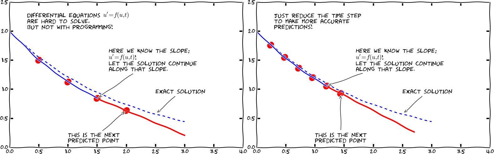
Soluzione con il metodo di Eulero
Un esempio di routine che risolve un'equazione differenziale in una variabile usando il metodo di Eulero:
# https://www.math.ubc.ca/~pwalls/math-python/differential-equations/first-order/

def odeEuler(f,y0,t):
    '''Approximate the solution of y'=f(y,t) by Euler's method.

    Parameters
    ----------
    f : function
        Right-hand side of the differential equation y'=f(t,y), y(t_0)=y_0
    y0 : number
        Initial value y(t0)=y0 wher t0 is the entry at index 0 in the array t
    t : array
        1D NumPy array of t values where we approximate y values. Time step
        at each iteration is given by t[n+1] - t[n].

    Returns
    -------
    y : 1D NumPy array
        Approximation y[n] of the solution y(t_n) computed by Euler's method.
    '''
    y = np.zeros(len(t))
    y[0] = y0
    for n in range(0,len(t)-1):
        y[n+1] = y[n] + f(y[n],t[n])*(t[n+1] - t[n])
    return y
y_E = odeEuler(f,y0,t)
import matplotlib.pyplot as plt         # plotting of results
fig, ax = plt.subplots()
ax.plot(t,y,label='sol by odeint')
ax.plot(t,y_E,c='r',label='sol by odeEuler')
ax.set_xlabel('t')
ax.set_ylabel('y(t)')
ax.legend()
Il comando odeint può prendere diversi parametri opzionali per modificare l'errore di default nell'integrazione (e per produrre output addizionale che può essere utile per il debugging). Usate il comando help per farvene un'idea:
help(scipy.integrate.odeint)
restituisce:
Help on function odeint in module scipy.integrate.odepack:

odeint(func, y0, t, args=(), Dfun=None, col_deriv=0, full_output=0, ml=None, mu=None, rtol=None, atol=None, tcrit=None, h0=0.0, hmax=0.0, hmin=0.0, ixpr=0, mxstep=0, mxhnil=0, mxordn=12, mxords=5, printmessg=0)
    Integrate a system of ordinary differential equations.

    Solve a system of ordinary differential equations using lsoda from the
    FORTRAN library odepack.

    Solves the initial value problem for stiff or non-stiff systems
    of first order ode-s::

        dy/dt = func(y, t0, ...)

    where y can be a vector.

    *Note*: The first two arguments of ``func(y, t0, ...)`` are in the
    opposite order of the arguments in the system definition function used
    by the `scipy.integrate.ode` class.

    Parameters
    ----------
    func : callable(y, t0, ...)
        Computes the derivative of y at t0.
    y0 : array
        Initial condition on y (can be a vector).
    t : array
        A sequence of time points for which to solve for y.  The initial
        value point should be the first element of this sequence.
    args : tuple, optional
        Extra arguments to pass to function.
    Dfun : callable(y, t0, ...)
        Gradient (Jacobian) of `func`.
    col_deriv : bool, optional
        True if `Dfun` defines derivatives down columns (faster),
        otherwise `Dfun` should define derivatives across rows.
    full_output : bool, optional
        True if to return a dictionary of optional outputs as the second output
    printmessg : bool, optional
        Whether to print the convergence message

    Returns
    -------
    y : array, shape (len(t), len(y0))
        Array containing the value of y for each desired time in t,
        with the initial value `y0` in the first row.
    infodict : dict, only returned if full_output == True
        Dictionary containing additional output information

        =======  ============================================================
        key      meaning
        =======  ============================================================
        'hu'     vector of step sizes successfully used for each time step.
        'tcur'   vector with the value of t reached for each time step.
                 (will always be at least as large as the input times).
        'tolsf'  vector of tolerance scale factors, greater than 1.0,
                 computed when a request for too much accuracy was detected.
        'tsw'    value of t at the time of the last method switch
                 (given for each time step)
        'nst'    cumulative number of time steps
        'nfe'    cumulative number of function evaluations for each time step
        'nje'    cumulative number of jacobian evaluations for each time step
        'nqu'    a vector of method orders for each successful step.
        'imxer'  index of the component of largest magnitude in the
                 weighted local error vector (e / ewt) on an error return, -1
                 otherwise.
        'lenrw'  the length of the double work array required.
        'leniw'  the length of integer work array required.
        'mused'  a vector of method indicators for each successful time step:
                 1: adams (nonstiff), 2: bdf (stiff)
        =======  ============================================================

    Other Parameters
    ----------------
    ml, mu : int, optional
        If either of these are not None or non-negative, then the
        Jacobian is assumed to be banded.  These give the number of
        lower and upper non-zero diagonals in this banded matrix.
        For the banded case, `Dfun` should return a matrix whose
        rows contain the non-zero bands (starting with the lowest diagonal).
        Thus, the return matrix `jac` from `Dfun` should have shape
        ``(ml + mu + 1, len(y0))`` when ``ml >=0`` or ``mu >=0``.
        The data in `jac` must be stored such that ``jac[i - j + mu, j]``
        holds the derivative of the `i`th equation with respect to the `j`th
        state variable.  If `col_deriv` is True, the transpose of this
        `jac` must be returned.
    rtol, atol : float, optional
        The input parameters `rtol` and `atol` determine the error
        control performed by the solver.  The solver will control the
        vector, e, of estimated local errors in y, according to an
        inequality of the form ``max-norm of (e / ewt) <= 1``,
        where ewt is a vector of positive error weights computed as
        ``ewt = rtol * abs(y) + atol``.
        rtol and atol can be either vectors the same length as y or scalars.
        Defaults to 1.49012e-8.
    tcrit : ndarray, optional
        Vector of critical points (e.g. singularities) where integration
        care should be taken.
    h0 : float, (0: solver-determined), optional
        The step size to be attempted on the first step.
    hmax : float, (0: solver-determined), optional
        The maximum absolute step size allowed.
    hmin : float, (0: solver-determined), optional
        The minimum absolute step size allowed.
    ixpr : bool, optional
        Whether to generate extra printing at method switches.
    mxstep : int, (0: solver-determined), optional
        Maximum number of (internally defined) steps allowed for each
        integration point in t.
    mxhnil : int, (0: solver-determined), optional
        Maximum number of messages printed.
    mxordn : int, (0: solver-determined), optional
        Maximum order to be allowed for the non-stiff (Adams) method.
    mxords : int, (0: solver-determined), optional
        Maximum order to be allowed for the stiff (BDF) method.

    See Also
    --------
    ode : a more object-oriented integrator based on VODE.
    quad : for finding the area under a curve.

    Examples
    --------
    The second order differential equation for the angle `theta` of a
    pendulum acted on by gravity with friction can be written::

        theta''(t) + b*theta'(t) + c*sin(theta(t)) = 0

    where `b` and `c` are positive constants, and a prime (') denotes a
    derivative.  To solve this equation with `odeint`, we must first convert
    it to a system of first order equations.  By defining the angular
    velocity ``omega(t) = theta'(t)``, we obtain the system::

        theta'(t) = omega(t)
        omega'(t) = -b*omega(t) - c*sin(theta(t))

    Let `y` be the vector [`theta`, `omega`].  We implement this system
    in python as:

    >>> def pend(y, t, b, c):
    ...     theta, omega = y
    ...     dydt = [omega, -b*omega - c*np.sin(theta)]
    ...     return dydt
    ...

    We assume the constants are `b` = 0.25 and `c` = 5.0:

    >>> b = 0.25
    >>> c = 5.0

    For initial conditions, we assume the pendulum is nearly vertical
    with `theta(0)` = `pi` - 0.1, and it initially at rest, so
    `omega(0)` = 0.  Then the vector of initial conditions is

    >>> y0 = [np.pi - 0.1, 0.0]

    We generate a solution 101 evenly spaced samples in the interval
    0 <= `t` <= 10.  So our array of times is:

    >>> t = np.linspace(0, 10, 101)

    Call `odeint` to generate the solution.  To pass the parameters
    `b` and `c` to `pend`, we give them to `odeint` using the `args`
    argument.

    >>> from scipy.integrate import odeint
    >>> sol = odeint(pend, y0, t, args=(b, c))

    The solution is an array with shape (101, 2).  The first column
    is `theta(t)`, and the second is `omega(t)`.  The following code
    plots both components.

    >>> import matplotlib.pyplot as plt
    >>> plt.plot(t, sol[:, 0], 'b', label='theta(t)')
    >>> plt.plot(t, sol[:, 1], 'g', label='omega(t)')
    >>> plt.legend(loc='best')
    >>> plt.xlabel('t')
    >>> plt.grid()
    >>> plt.show()
Imparare Facendo
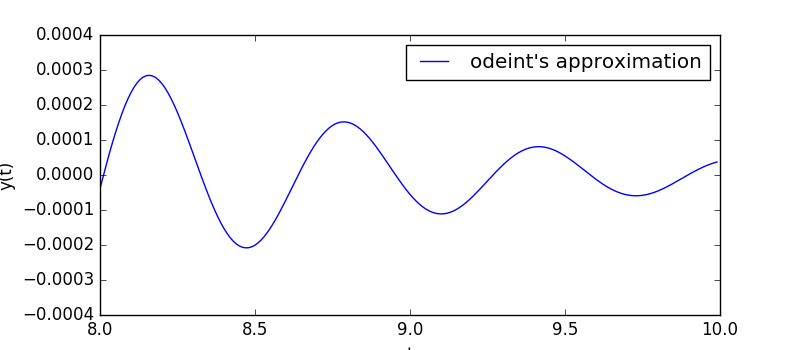
Scrivete un programma che calcoli la soluzione y(t) della ODE seguente, usando l'algoritmo odeint,
$$\frac{\mathrm{d}y}{\mathrm{d}t} = -\exp(-t)(10\sin(10t)+\cos(10t))$$
da $t=0$ a $t = 10$. Il valore iniziale è $y(0)=1$.
Mostrate graficamente la soluzione, valutandola nei punti $t=0$, $t=0.01$, $t=0.02$, ..., $t=9.99$, $t=10$.
Aiutino: una parte della soluzione $y(t)$ è presentata nella figura seguente.
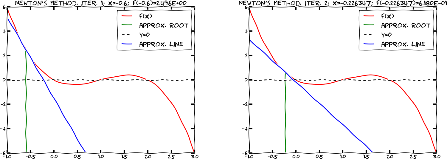
10.4 Ricerca delle radici
Cercare una $x$ tale che $f(x)=0$ si chiama ricerca delle radici di $f$. Si noti che un problema del tipo $g(x)=h(x)$ può essere riformulato come $f(x)=g(x)−h(x)=0$.
Il modulo optimize di scipy fornisce diversi strumenti per la ricerca delle radici.
(Svein Linge, Hans Petter Langtangen - Programming for Computations)
Ricerca delle radici usando il metodo della bisezione
L'algoritmo bisect è (i) robusto e (ii) concettualmente molto semplice (ma lento).
Supponiamo di dover calcolare le radici di $f(x)= x^3 − 2 x^2$. Questa funzione ha una radice (doppia) in $x = 0$ e un'altra fra $x = 1.5$ (dove $f(1.5) = − 1.125$) e $x = 3$ (dove $f(3) = 9$). È facile vedere che questa altra radice si trova in $x = 2$. Ecco il programma che determina la radice numericamente:
from scipy.optimize import bisect

def f(x):
    """returns f(x)=x^3-2x^2. Has roots at
    x=0 (double root) and x=2"""
    return x ** 3 - 2 * x ** 2

# main program starts here. Typically, the range in which to perform the search is determined from a plot.
x = bisect(f, 1.5, 3, xtol=1e-6)

print(f"The root x is approximately x={x:14.12g},\n"
      f"the error is less than 1e-6.")
print(f"The exact error is {2 - x:g}.")
Il metodo bisect() richiede obbligatoriamente tre argomenti: (i) la funzione f(x), (ii) il limite inferiore a (che abbiamo scelto uguale a 1.5 nell'esempio) e (ii) il limite superiore b (scelto uguale a 3) dell'intervallo in cui eseguire la procedura. Il parametro opzionale xtol determina l'errore massimo del metodo.
Uno dei presupposti del metodo di bisezione è che l'intervallo [a, b] sia scelto in modo tale che la funzione abbia in a segno opposto a quello che ha in b in modo che nell'intervallo, se la funzione è continua, cada almeno una radice.
Imparare Facendo
Scrivete un programma chiamato sqrttwo.py per cercare la radice x della funzione $f(x)=2 − x^2$ usando il metodo di bisezione. Scegliete come tolleranza per l'approssimazione alla radice 10−8.
- Giustificate la scelta dell'intervallo iniziale $[a, b]$ per la ricerca: che valori evte scelto per *a* e *b*? Perchè?
- Esaminate i risultati:
- Che valore restituisce l'algoritmo di bisezione per la radice *x*?
- Calcolate il valore di $\sqrt{2}$ usando math.sqrt(2) e confrontatelo il risultato precedente. Quanto è grande l'errore assoluto? Come si confronta con xtol?
Ricerca delle radici usando la funzione fsolve
Un algoritmo per la ricerca delle radici che è (spesso) migliore (nel senso di “più efficiente”) di quello di bisezione è codificato nella funzione fsolve() che funziona anche per problemi a più dimensioni. Questo algoritmo richiede solamente un punto di partenza vicino a dove ci si aspetta che ci sia una radice (Non è però detto che il metodo converga).
Ecco un esempio:
from scipy.optimize import fsolve

def f(x):
    return x ** 3 - 2 * x ** 2

xstart = 3
x = fsolve(f, xstart)      # one root is at x=2.0
                           # search starts at x=3
                           # fsolve returns a numpy array

print(f"The root x is approximately x={x[0]:21.19g}")
print(f"The exact error is {2 - x[0]:g}.")
Il valore restituito da fsolve è un array di numpy di lunghezza $n$ per un problema di ricerca di radici con $n$ variabili. Nell'esempio precedente, $n = 1$.
Imparare Facendo
- Studiate il grafico della funzione y(x) = np.cos(2*x) - np.cosh(-x+1) + 2, cambiando l'intervallo di variazione dell'ascissa fino determinare il numero e la posizione approssimata degli zeri. Trovate il valore degli zeri usando fsolve
10.5 Fit di un set di dati
Scipy fornisce una funzione piuttosto flessibile (basato sull'algoritmo di Levenburg-Marquardt), scipy.optimize.curve_fit, per interpolare un set di dati. L'assunzione è che vengano dati un set di punti
$x_1, x_2,\cdots,x_N$, i corrispondenti valori $y_i$ e una dipendenza funzionale $y=f(x,\vec{p})$.
Per fare un esempio, il numero di atomi non decaduti in un campione di una sostanza radioattiva segue la legge
$$ N(t,N_0,\tau) = N_0\,\exp\left(-\frac{t}{\tau}\right).$$
Si vuole determinare i parametri $\vec{p}=(p_1, p_2, \ldots,p_k)$ in modo che $r$, la somma degli scarti quadratici fra la curva e i dati, sia la più piccola possibile:
Questo approccio è particolarmente utile quando i dati sono affetti da rumore: per ogni coppia $x_i,y_i$ è presente un termine di errore (ignoto) $\epsilon_i$, tale che $y_i=f(x_i,\vec{p})+\epsilon_i$.
Un esempio per chiarire: assumiamo di avere dei dati che sappiamo essere descritti dalla funzione: $$f(x,\vec{p}) = a \exp(-b x) + c,$$ che dipende dai parametri $\vec{p}=(a,b,c)$, che devono essere determinati usando i dati.
import numpy as np
from scipy.optimize import curve_fit


def f(x, a, b, c):
    """Fit function y=f(x,p) with parameters p=(a,b,c). """
    return a * np.exp(- b * x) + c

#create fake data
x = np.linspace(0, 4, 50)
y = f(x, a=2.5, b=1.3, c=0.5)
#add noise
yi = y + 0.2 * np.random.normal(size=len(x))

#call curve fit function
popt, pcov = curve_fit(f, x, yi)
# extract fit parameters
af, bf, cf = popt
print(f"Optimal parameters are af={af:g}, bf={bf:g}, and cf={cf:g}.")

# best fit curve
yfitted = f(x,af,bf,cf)

#plot
import matplotlib.pyplot as plt
fig, ax = plt.subplots(figsize=(6,4))
ax.scatter(x, yi, marker='o', label='data $y_i$')
ax.plot(x, yfitted, c='r', label='fit $f(x_i)$')
ax.set_xlabel('x')
ax.legend()
Si noti che nell'esempio precedente abbiamo definito la funzione da utilizzare per il fit $y = f(x)$ usando del codice Python. Quindi possiamo utilizzare una funzione (quasi) arbitraria nel metodo curve_fit.
La funzione curve_fit restituisce una tuple popt, pcov. Il primo elemento, popt, contiene l'ntupla dei parametri ottimali (OPTimal Parameters), cioè i parametri che minimizzano la somma degli scarti quadratici. Il secondo elemento, pcov, contiene la matrice di covarianza di tutti i parametri (Sperimentazioni di Fisica). La diagonale fornisce la varianza della stima dei parametri. La standard deviation sulla stima dei parametri può quindi essere calcolata come
perr = np.sqrt(np.diag(pcov)).
L'algoritmo di Levenburg-Marquardt richiede, per iniziare la sua procedura, una stima iniziale dei parametri. Se questa non viene fornita, come nell'esempio precedente, il valore “1.0“ viene assunto come stima di partenza.
Se l'algoritmo non riesce a fittare i dati con la funzione ipotizzata, è necessario fornire a curve_fit una stima migliore per i parametri iniziali. Nell'esempio precedente potremmo passare le nostre stime cambiando la linea
popt, pcov = curve_fit(f, x, yi)
in
popt, pcov = curve_fit(f, x, yi, p0=(2,1,0.6))
se avessimo ragione di ritenere che a = 2, b = 1 and c = 0.6 siano dei valori "ragionevoli". Una volta che la stima iniziale è "più o meno corretta" il fit funziona bene.
Imparare Facendo
Un set di misure ha dato il risultato
array([ 1.98781717e-01,  3.24825975e-01,  2.98912925e-01,  4.93741345e-02,
  3.80536122e-01, -2.05719267e-01, -7.71630572e-03, -1.51733833e-01,
  1.73748896e-02,  9.02509179e-03, -2.20920245e-02,  1.34501550e-02,
  3.06908554e-01,  2.34147443e-01,  7.75703310e-01,  4.99104499e-01,
  5.66648179e-01,  1.04641129e+00,  1.67507051e+00,  1.77283086e+00,
  1.96239227e+00,  2.27163706e+00,  2.54161451e+00,  3.09807009e+00,
  3.45291476e+00,  4.23653254e+00,  4.58924190e+00,  5.08824411e+00,
  5.76377627e+00,  6.04351916e+00,  6.59161494e+00,  7.25319841e+00,
  7.96917169e+00,  8.06559558e+00,  8.91595385e+00,  9.78458262e+00,
  1.04143742e+01,  1.14280612e+01,  1.18132229e+01,  1.25599940e+01,
  1.35895984e+01,  1.41159890e+01,  1.53848688e+01,  1.63810995e+01,
  1.69877641e+01,  1.77683845e+01,  1.88923474e+01,  1.95531287e+01,
  2.12809123e+01,  2.15518168e+01])
ai tempi
array([0.        , 0.10204082, 0.20408163, 0.30612245, 0.40816327,
       0.51020408, 0.6122449 , 0.71428571, 0.81632653, 0.91836735,
       1.02040816, 1.12244898, 1.2244898 , 1.32653061, 1.42857143,
       1.53061224, 1.63265306, 1.73469388, 1.83673469, 1.93877551,
       2.04081633, 2.14285714, 2.24489796, 2.34693878, 2.44897959,
       2.55102041, 2.65306122, 2.75510204, 2.85714286, 2.95918367,
       3.06122449, 3.16326531, 3.26530612, 3.36734694, 3.46938776,
       3.57142857, 3.67346939, 3.7755102 , 3.87755102, 3.97959184,
       4.08163265, 4.18367347, 4.28571429, 4.3877551 , 4.48979592,
       4.59183673, 4.69387755, 4.79591837, 4.89795918, 5.        ])
Trovate la parabola della forma
y(t) = a*t**2 + b*t + c
che meglio approssima i dati.Fate un plot dei dati e della curva ottenuta.
10.6 Ottimizzazione ovvero trovare minimi (e massimi)
Spesso è necessario trovare il minimo o il massimo di una particolare funzione f(x) dove f è una funzione scalare mentre x può essere un vettore. Applicazioni tipiche sono la minimizzazione di quantità come il costo, il rischio o l'errore, oppure la massimizzazione della produttività, efficienza o profitto. Le routines di ottimizzazione tipicamente forniscono un metodo per minimizzare una funzione data: per massimizzare f(x) è sufficiente minimizzare g(x)= − f(x).
Di seguito, un esempio che mostra (i) la definizione della funzione f(x) da minimizzare e (ii) la chiamata a scipy.optimize.fmin a cui vengono passati la funzione f da minimizzare e un valore iniziale x0 da cui partire per la ricerca del minimo, e che restituisce il valore x per cui f(x) ha un minimo locale. Tipicamente, la ricerca del minimo è locale, nel senso che l'algoritmo segue il gradiente (derivata multidimensionale) nel punto in cui si trova.
Facciamo come prima cosa il grafico della funzione. Il plot suggerisce che i due minimi più a destra possono essere cercati partendo dai due punti x0 = 1.0 e x0 = 2.0.
import numpy as np
from scipy.optimize import fmin
import matplotlib.pyplot as plt

def f(x):
    return np.cos(x) - 3 * np.exp( -(x - 0.2) ** 2)


# plot function
x = np.arange(-10, 10, 0.1)
y = f(x)

fig, ax = plt.subplots(figsize=(6,4))
ax.set_xlabel('x')
ax.grid(visible=True,which='both')
ax.set_xlim(-5.,5.)
ax.set_ylim(-2.2,0.5)

ax.plot(x, y, label='$\cos(x)-3e^{-(x-0.2)^2}$')
Troviamo i due minimi con due chiamate a fmin. Il risultato mostra come, in generale, partendo da punti diversi troviamo minimi diversi. È anche possibile che esistano punti iniziali che non portano a nessun minimo. Rigeneriamo il plot della funzione, mostrando i punti iniziali delle due ricerche e i minimi ottenuti:
# find minima of f(x),
# starting from 1.0 and 2.0 respectively
minimum1 = fmin(f, 1.0)
print("Start search at x=1., minimum is", minimum1)
minimum2 = fmin(f, 2.0)
print("Start search at x=2., minimum is", minimum2)

# plot function again showing the minima that have been found
x = np.arange(-10, 10, 0.1)
y = f(x)

fig, ax = plt.subplots(figsize=(6,4))
ax.set_xlabel('x')
ax.grid(visible=True,which='both')
ax.set_xlim(-5.,5.)
ax.set_ylim(-2.2,0.5)

ax.plot(x, y, label='$\cos(x)-3e^{-(x-0.2)^2}$')
# add minimum1 to plot
ax.scatter(minimum1, f(minimum1), marker='v', c='r', label='minimum 1')
# add start1 to plot
ax.scatter(1.0, f(1.0), marker='o', c='r', label='start 1')

# add minimum2 to plot
ax.scatter(minimum2,f(minimum2), marker='v', c='g', label='minimum 2')
# add start2 to plot
ax.scatter(2.0,f(2.0), marker='o', c='g',label='start 2')

ax.legend(loc='lower left')
Come si vede, la chiamata a fmin produce anche dell'output addizionale che può essere utile per analizzare la procedura.
Valori ritornati da fmin
Si noti che la funzione fmin restituisce un numpy array che – nel caso precedente – contiene un solo numero dal momento che abbiamo una sola variabile (qui x) da variare. In generale, fmin può essre usata per trovare il minimo in uno spazio pluridimensionale. In questo caso, il numpy array contiene le coordinate del punto che minimizza la funzione obiettivo.
Imparare Facendo
- Trovate massimi e minimi della funzione $f(x) = 2\, x^3 + 3\, x^2 - 12\, x - 10$.
- Trovate la distanza minima fra il punto del piano (3,2) e la retta y = 3x -1.
Altri metodi numerici
Scientific Python and Numpy forniscono molti altri algoritmi numerici: per esempio interpolazione di funzioni, trasformate di Fourier, funzioni speciali (Funzioni di Bessel etc.), signal processing e filtri.
Ulteriori informazioni ed esempi:
Scipy-lectures.
Robert Johansson - Scientific Computing with Python
Sven Linge, Hand Petter Langtangen - Programming for Computations
Sommario 10: Metodi Numerici in Python (SciPy)
La libreria SciPy, basata su NumPy, fornisce numerosi algoritmi per l'elaborazione scientifica.
Integrazione numerica
scipy.integrate.quad() è la routine base per calcolare integrali definiti in una variabile su intervalli finiti o infiniti.
Integrazione con parametri
Le funzioni che dipendono da parametri possono essere integrate passando i parametri come argomenti extra a quad() con la keyword args.
Metodi dei trapezi e di Simpson
Sono disponibili routines che implementano specifici metodi di integrazione come il metodo dei trapezi (trapezoid()) e il metodo di Simpson (simpson()).
Risoluzione di Equazioni Differenziali Ordinarie (ODE)
Le equazioni differenziali ordinarie (ODE) di ordine n possono essere riscritte come un sistema di equazioni differenziali di primo ordine. La libreria scipy fornisce una funzione chiamata odeint per risolvere queste equazioni.
Ricerca delle radici
Sono disponibili diversi metodi per la ricerca delle radici di una funzione nel modulo scipy.optimize.
Metodo di Bisezione
L'algoritmo bisect è robusto e semplice, anche se non molto veloce. Il metodo richiede che la funzione abbia segni opposti ai due estremi dell'intervallo in cui la radice viene cercata.
Metodo fsolve
Un metodo alternativo, spesso più efficiente, è fsolve. Richiede solo un punto di partenza vicino alla radice attesa e funziona anche con problemi multi-dimensionali.
Fit di un set di dati
SciPy fornisce la funzione curve_fit per effettuare il fit di un set di dati basato su un modello ipotizzato. Questo approccio minimizza la somma degli scarti quadratici tra i dati e la curva.
Ottimizzazione: trovare massimi e minimi
La routine scipy.optimize.fmin permette di minimizzare una funzione f(x). Per massimizzare una funzione, è sufficiente minimizzare -f(x).