


Next: Smooth-filamental transition
Up: Passive scalar with finite
Previous: Chaotic advection and linear
Contents
The previous results which has been presented with intuitive
but not-rigorous arguments, are formally valid only in a mean field sense,
i.e. assuming a constant stretching rate  .
This is not the general case.
.
This is not the general case.
While in the limit of infinite time the stretching rate
is the same for almost all trajectories in an ergodic region,
and is given by the Lyapunov exponent,
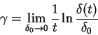
the stretching rates at a finite time  are given by
the finite time Lyapunov exponents
are given by
the finite time Lyapunov exponents  ,
which are defined as
,
which are defined as
 |
(2.17) |
Because of their local character they
can assume different values depending on the initial positions
of the trajectories along which they are measured.
For large their distribution approaches the asymptotic form
![\begin{displaymath}
P(\gamma,t) \sim t^{1/2} \exp[-S(\gamma) t]
\end{displaymath}](img327.png) |
(2.18) |
The Cramér function  (also called entropy function)
is concave, positive, with a quadratic minimum in
(the maximum Lyapunov exponent)
(also called entropy function)
is concave, positive, with a quadratic minimum in
(the maximum Lyapunov exponent)  , and
its shape far from the minimum depends on the details of
the velocity statistics [38,39].
The quadratic minimum of correspond to a
Gaussian behavior for the core of the probability
distribution of the stretching rate , which
can be predicted in the general case thanks
to the Central Limit Theorem.
In the limit
, and
its shape far from the minimum depends on the details of
the velocity statistics [38,39].
The quadratic minimum of correspond to a
Gaussian behavior for the core of the probability
distribution of the stretching rate , which
can be predicted in the general case thanks
to the Central Limit Theorem.
In the limit  the distribution became a
  -distribution
with support for
-distribution
with support for
 .
.
Local fluctuations of the stretching rates are the origin of the
intermittent behavior of the passive scalar statistic.
Indeed, in order to obtain the correct evaluation of the
structure functions of passive scalar fluctuations,
it is necessary to average over the distribution
of finite-time Lyapunov exponents:
![\begin{displaymath}
S^{\theta}_p (r) \equiv \langle (\delta_r \theta)^p \rangle ...
...]/\gamma}
\sim \left({r \over L} \right)^{\zeta^{\omega}_p}\;.
\end{displaymath}](img331.png) |
(2.19) |
The scaling exponents are evaluated from Eq. (2.20)
by a steepest descent argument as:
![\begin{displaymath}
\zeta^{\theta}_p = \min_{\gamma} \left\{
p,[p \alpha + S(\gamma)]/\gamma \right\}\;.
\end{displaymath}](img332.png) |
(2.20) |
Intermittency manifests itself in the nonlinear dependence
of the exponents
 on the order
  .
.
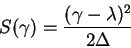
In the Gaussian approximation for  , which holds
near its core, the Cramér function has the quadratic expression:
, which holds
near its core, the Cramér function has the quadratic expression:
 |
(2.21) |
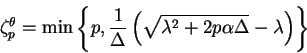
and it is possible to obtain an explicit expression for the
scaling exponents
 :
:
 |
(2.22) |
Next: Smooth-filamental transition
Up: Passive scalar with finite
Previous: Chaotic advection and linear
Contents
Stefano Musacchio
2004-01-09