


Next: Statistics of velocity fluctuations
Up: Active polymers
Previous: Depletion of kinetic energy
Contents
Energy balance
The suppression of velocity fluctuations by polymer additives
in two-dimensional turbulence can be easily explained
in the context of the randomly driven viscoelastic model.
Indeed, the average kinetic energy balance
in the statistically stationary state reads
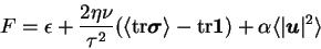 |
(4.17) |
where
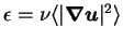 is
the viscous dissipation and
is
the viscous dissipation and  is the average energy input,
which is flow-independent for a Gaussian,
is the average energy input,
which is flow-independent for a Gaussian,  -correlated
random forcing
-correlated
random forcing
 .
To obtain Eq. (4.17) we multiply Eq. (4.1) by
.
To obtain Eq. (4.17) we multiply Eq. (4.1) by
 ,
add to it the trace of Eq. (4.2) times
,
add to it the trace of Eq. (4.2) times  ,
and average over space and time.
Since in two dimensions kinetic energy flows towards large scales,
it is mainly drained by friction, and
viscous dissipation is vanishingly small in the limit of
very large Reynolds numbers [71].
Neglecting
,
and average over space and time.
Since in two dimensions kinetic energy flows towards large scales,
it is mainly drained by friction, and
viscous dissipation is vanishingly small in the limit of
very large Reynolds numbers [71].
Neglecting  and observing that
in the Newtonian case (
and observing that
in the Newtonian case ( ) the balance (4.8)
yields
) the balance (4.8)
yields
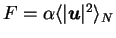 ,
we obtain
,
we obtain
 |
(4.18) |
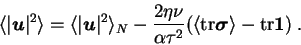
According to Eq (4.11), incompressibility of the flow ensures that
 , and we finally have
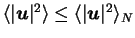 ,
in agreement with numerical results.
This simple energy balance argument can be generalized to nonlinear
elastic models. As viscosity tends to zero,
the average polymer elongation increases so as to compensate for the
factor
,
in agreement with numerical results.
This simple energy balance argument can be generalized to nonlinear
elastic models. As viscosity tends to zero,
the average polymer elongation increases so as to compensate for the
factor  in eq. (4.18), resulting in a finite effect
also in the infinite
in eq. (4.18), resulting in a finite effect
also in the infinite  limit.
Since energy is essentially dissipated by linear friction, the depletion
of
limit.
Since energy is essentially dissipated by linear friction, the depletion
of
 entails immediately the reduction
of energy dissipation. The main difference between two-dimensional
``friction reduction'' and three-dimensional drag reduction
resides in the lengthscales involved in the energy drain, i.e.
large scales in 2D vs small scales in 3D.
entails immediately the reduction
of energy dissipation. The main difference between two-dimensional
``friction reduction'' and three-dimensional drag reduction
resides in the lengthscales involved in the energy drain, i.e.
large scales in 2D vs small scales in 3D.
Next: Statistics of velocity fluctuations
Up: Active polymers
Previous: Depletion of kinetic energy
Contents
Stefano Musacchio
2004-01-09